
Originally Posted by
jaydee49

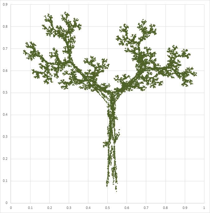
Hi, I'm fascinated by your work on excel and upon looking at your spreadsheet for the Barnsley fern I'm still a little bit confused about the formulas you have used to generate your data that excel uses to plot the graph of the ifs. Any chance of a quick explanation of the formulas of each column?
Many thanks
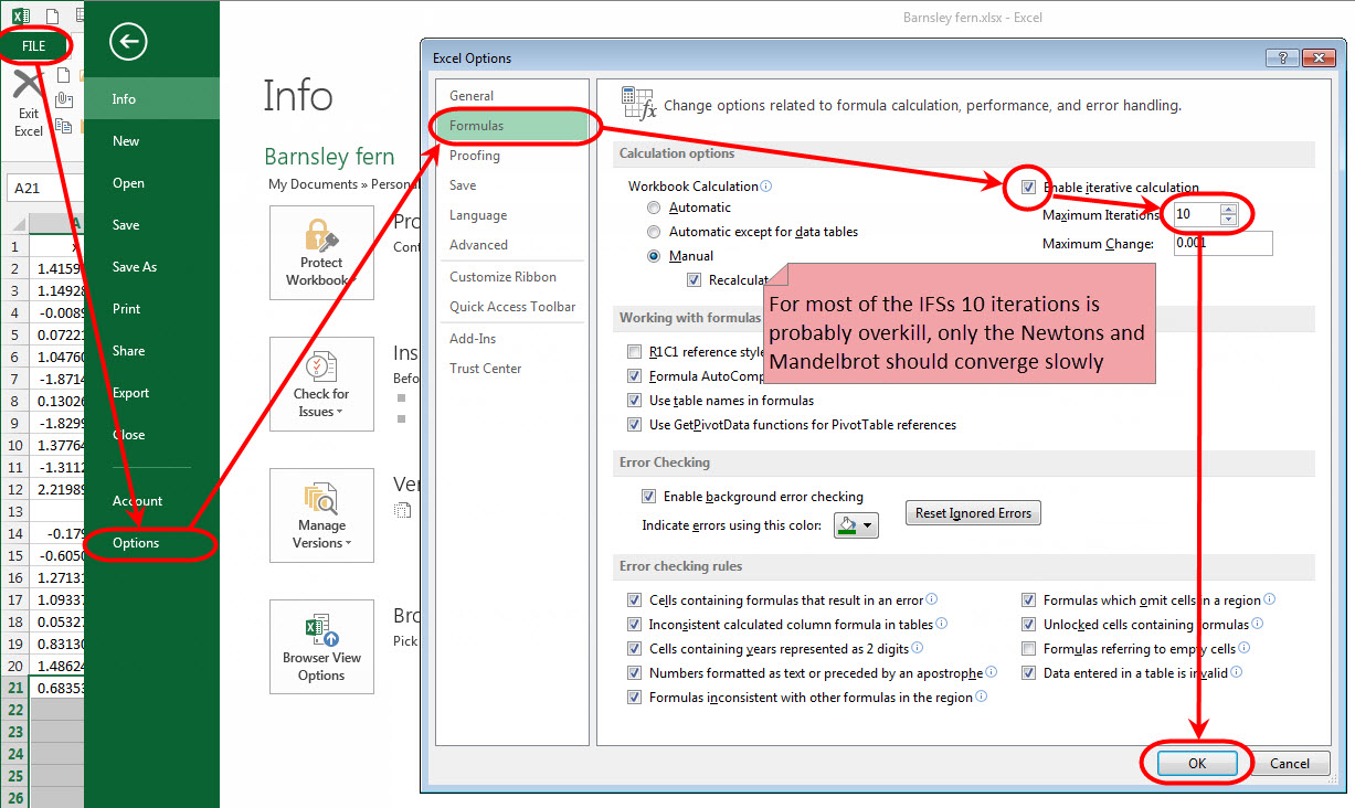
Sure however first you'll need to switch your Excel into Iterative calculation mode for the formulas to work.

M1, this cell resets the calculation loops for columns A and B if set to TRUE

Column A: =IF($M$1,RAND(),C2)
if M1 is
     true: then gives a new random number in the interval [0,1)
     false: then gives the value of C2 (which is the value after the affine chosen by E2 has been applied)

Column B: =IF($M$1,RAND(),D2)
same as A except for they y value

Column C: =INDEX($K$4:$K$7,E2)*A2+INDEX($L$4:$L$7,E2)*B2+INDEX($O$4:$O$7,E2)
uses the affine chosen by E2 to transform the x value
INDEX($K$4:$K$7,E2)
if E2 is
    1: then value of K4
    2: then value of K5
    3: then value of K6
    4: then value of K7
a*A2+b*B2+e is the generic affine transform, where the a b and e values come from K4:P7

Column D: =INDEX($M$4:$M$7,E2)*A2+INDEX($N$4:$N$7,E2)*B2+INDEX($P$4:$P$7,E2)
same as C except transforms the y value

Column E: =COUNTIF($U$4:$U$7,"<"&RAND())+1+0*D2
select which affine transform to use based on the probability density formula(PDF) given in U4:U7
RAND() gives a value in the semi-open interval [0,1)
COUNTIF counts the number of values in this case "<" my RAND()
if RAND() is
   0<= RAND() < 0.05 then COUNTIF is 0
   0.05<= RAND() < 0.05+0.72 then COUNTIF is 1
   0.05+0.72<= RAND() < 0.05+0.72+.10 then COUNTIF is 2
   0.05+0.72+.10<= RAND() < 1 then COUNTIF is 3
COUNTIF()+1 moves the index range from [0,3] to [1,4]
+0*D2 this forces the calculation of this formula to happen on each iteration

(ok at this point i should note what the iteration is doing, the formulas in column A point
 to column C and the formulas in C point to A thus creating a loop. Excel usually doesn't
like that so much, but with iterative calulation turned on it's ok because it will not loop
forever, just the number of times you specified in the options. So Excel starts with A does
its calcs based on the current stat moves to C does its calcs moves to A redoes its calcs
based on the new values of C, moves to C does its calcs based on the new values of A and so
on in a loop until the iteration count is reached. Likewise with B pointing to D pointing
to B, also C and D both point to E which points to D so that it's included on the ride too.)

Column J: just the formula naming convention
Column K: the a coefficients for the affine transforms
Column L: the b coefficients for the affine transforms
Column M: the c coefficients for the affine transforms
Column N: the d coefficients for the affine transforms
Column O: the e coefficients for the affine transforms
Column P: the f coefficients for the affine transforms
Column Q: the typical probabilities (typical PDF)
Column R: simple descriptions of which piece of the picture the affine represents
Column S: determinate of the affine's matrix, S1 is a hard coded value
Column T: my probabilities based on the coverage of the affine (my PDF)
Column U: the running total of the probabilites used by E to select which affine to use


 LinkBack URL
 About LinkBacks


 |a b| |x| |e|
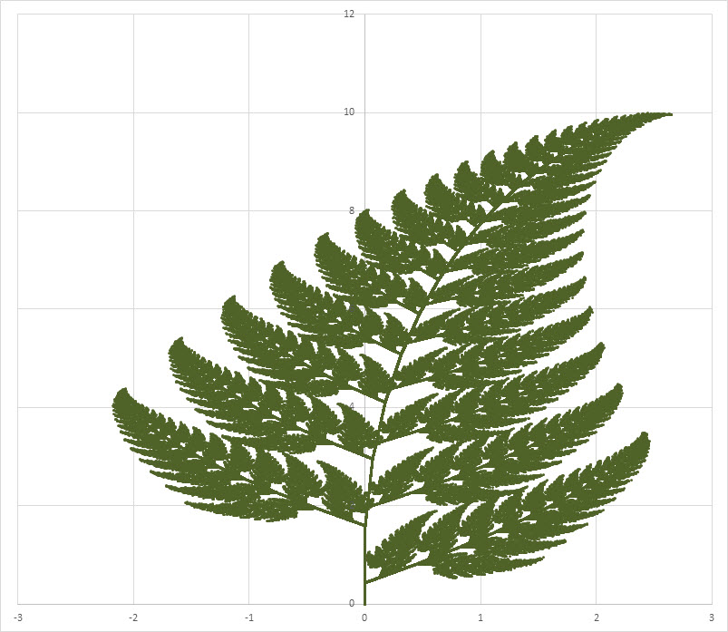

 Add Reputation
 Register To Reply

 below the post.


Bookmarks