Advanced VLOOKUP

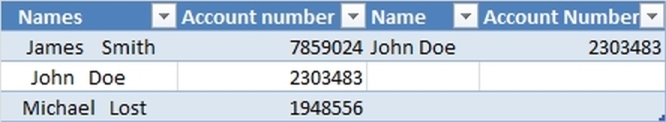
The VLOOKUP function is, IMHO, one of the most used functions in Excel. Even so, spelling mistakes and extra spaces can throw it off completely. Here's my simple solution for dealing with extra spaces.

Tip #1)
N.B. Intentional extra spaces have been put before, in the middle, and after each name:

Instead of:

Formula:

=VLOOKUP(D2,A1:B4,2,0)

You can use:

Formula:

=VLOOKUP(TRIM(D2),TRIM(A1:B4),2,0)

entered as Ctrl+Shift+Enter

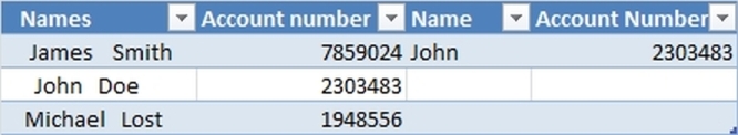
Tip #2)
Now you might only know one name (e.g. John or Doe) but not the other name (ie. partial match). Then you can use a little semi-fuzzy logic to get the answer:

Formula:

=VLOOKUP("*"&TRIM(D3)&"*",A1:B4,2,0)

N.B. The above formula assumes that you are only looking up one word (e.g. no spaces).

If you are looking for a partial match with more than one word (e.g. Joh D) then use this formula:

Formula:

=VLOOKUP("*"&TRIM(D2)&"*",TRIM(A1:B4),2,0) 

entered as Ctrl+Shift+Enter

Tip #3)
If you are having problems with spelling mistakes, etc. then you need to get really fuzzy. Alan has provided some awesome code for doing Fuzzy-VLookup including Soundex and Metaphone similarities.

If your boss is against using non-Microsoft add-ins or vba macros/functions then you can rest assured that MS has jumped on the bandwagon and now has its own version of Fuzzy matching for VLookup. You can find the add-in here, but be warned that it only works on tables and only officially with Excel 2010. Debra has created a page on this topic and one of the comments posted is that it also works on Excel 2007. Haven't tried it except on Excel 2010 so can't comment.

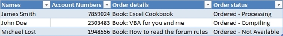
Tip #4)
One of the greatest limitations of VLookup is that is only looks up in one direction (to the right) of any said value. Looking at the example below, if you wanted to use an account number to find out the rest of the details of a purchase you woud not be able to do so with the traditional vlookup formula since the account numbers are not the first column in the lookup table.

This tip is actually two in one:

Part 1. If you only wanted to know one piece of information that is related to your lookup value then you can use a combination of Choose and VLookup:

Formula:

=VLOOKUP(F2,CHOOSE({1,2},B2:B4,A2:A4),2,0)

this tricks vlookup into switching the columns around and so finds the account number in Column B and returns the associated value from Column A. This technique is detailed here (http://www.myonlinetraininghub.com/e...t-using-choose).

Part 2. Often this is not enough and you would like to be build a complete retrieval system for the information in the VLookup table as you would with a traditional VLookup formula. This can be accomplished by taking the above formula one step further by creating a nested VLookup formula where the inner VLOOKUP will provide the lookup value for the outer VLOOKUP. If anyone knows of any references for this I will be happy to post it as I actually thought of this by myself (not saying I was the first, but I haven't seen anyone else use this technique before).

Names:

Formula:

=VLOOKUP(F2,CHOOSE({1,2},B2:B4,A2:A4),2,0)

Order details:

Formula:

=VLOOKUP(VLOOKUP(F2,CHOOSE({1,2},B2:B4,A2:A4),2,0),A2:D4,3,0)

Order status:

Formula:

=VLOOKUP(VLOOKUP(F2,CHOOSE({1,2},B2:B4,A2:A4),2,0),A2:D4,4,0)

Hope this helps.

abousetta

Of course any suggestions on improvement are highly desirable and welcomed.

Thanks.

abousetta

Thanks Cutter. You are right.

Thanks Cutter, I have amended my earlier post. I think the issue is that I can't see the 'Like' button for my own posts and that's why I was confused.

Thanks again for the vote.

abousetta

Hi,

In tip #2 the

=VLOOKUP("*"&TRIM(D2)&"*",TRIM(A1:B4),2,0)

You don't need the TRIM(A1:B4) as the "*Trim(D2)*" doesn't care if it is trimmed or not.

Good point Marvin. I have updated Tip #2.

Not necessarily - TRIM also removes excessive spaces between words, not just at the beginning and end.

Thanks for that RS. In fact we are all right depending on the lookup value (single word versus multiple words). I have returned the version using trim as a variant.

@abousetta,

Beware of the TRIM() function. In some programs and/or versions it DOES NOT reduce multiple spaces to a single space when "inside" the string. I would need to research this a little more but I believe older versions of Excel didn't reduce double spaces to a single. I would also worry about VBA vs Excel TRIM(). Anybody up for running this down? I also believe there are little differences between Access and Excel with this middle spaces question.

I heard about the difference between Excel function Trim and vba Trim. vba Trim only clears the leading and end spaces, while the function removes multiple spaces between words also. It was even suggested in a previous post by one of the MVPs to use application.trim() in vba if the need appears.

As for using it in earlier versions, I don't know about any changes made to this function during the version upgrades, but it is possible.

Two new tips have been added to the first post along with pics and a sample workbook.

Hope this helps.

abousetta

This post is only to allow me to show the figures in post #1

This post is only to allow me to show the figures in post #1

OK. I think the pics are now visible in the first post. If anyone can't see them, then please let me know and I will investigate it further.

Thanks.

abousetta

You can also add VLOOKUP function using range within a function:

Formula:

=VLOOKUP(A1,{"a"\2,"b"\3,"c"\4},2,FALSE)

Hi Zbor,

Could you explain this a bit because I'm not sure I understand the formula you posted? Also it's giving me an error (in error):

Formula:

=VLOOKUP(A1,{"a"\2,"b"\3,"c"\4},2,FALSE)

Thanks.

abousetta

Originally Posted by abousetta

Hi Zbor,
Could you explain this a bit because I'm not sure I understand the formula you posted? Also it's giving me an error (in error):

There could be regional setting problem. In above I just replace ; with , but maybe you need to adopt something more.
Here is original formula:

Formula:

=VLOOKUP(A1;{"a"\2\"test";"b"\3\"untest";"c"\4\"testing"};3;FALSE)

With c in A1 it return testing as expected.

Thanks zbor, yes I fiddled with it until I got the regional settings correctly

Formula:

=VLOOKUP(A1,{"a",2,"test";"b",3,"untest";"c",4,"testing"},2,FALSE)

Thanks Pete. I will add this tip also to the first post.

abousetta

Thanks for the feedback. I'm glad that the effort is well-received.

abousetta

Unfortunately your post does not comply with Rule 2 of our Forum RULES. Do not post a question in the thread of another member -- start your own thread.

If you feel an existing thread is particularly relevant to your need, provide a link to the other thread in your new thread.

Old threads are often only monitored by the original participants. New threads not only open you up to all possible participants again, they typically get faster response, too.